Let’s first import a few useful libraries:
import numpy as np
import scipy
from scipy.io import loadmat
import matplotlib.pyplot as plt
import matplotlib.cm as cm
from matplotlib.animation import FuncAnimation
%matplotlib inline
from sklearn.model_selection import train_test_split
from IPython.display import HTML
Simulation results are stored in a Matlab file with a .mat format. We’re
interested in finding a lower dimensional decomposition of the vorticity defined
as
\(\boldsymbol \omega = \nabla \times \mathbf u\)
where \(\mathbf u\) is the velocity field with two components \(\mathbf u = [u,
v]\). Let’s first plot the vorticity
results = loadmat('cyl_flow_data.mat')
m = int(results['m'][0][0])
n = int(results['n'][0][0])
v = results['VALL'][:, 0].reshape((n, m))
u = results['UALL'][:, 0].reshape((n, m))
vort0 = results['VORTALL'][:, 0].reshape((n, m))
tsteps = results['VORTALL'].shape[1]
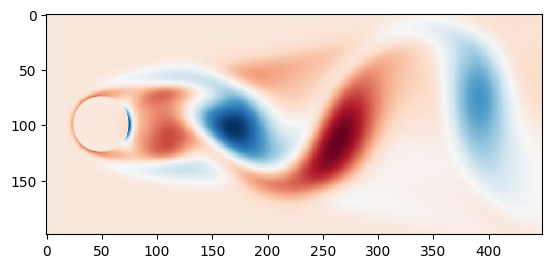
Use imshow for plotting the vorticity at \(t=0\)
vortmean = np.mean(results['VORTALL'], axis=1).reshape((n, m)).T
plt.imshow(vort0.T - vortmean, cmap=cm.RdBu, interpolation='none')
plt.show()
We can also look at the whole simulation by using the matplotlib.animation library
fig = plt.figure()
ax = fig.add_subplot(111)
im = ax.imshow(vort0.T - vortmean, cmap=cm.RdBu)
# vortmean = np.mean(vort, axis=2)
# update the frames based on the parameter i
def animate(i):
vort = results['VORTALL'][:, i].reshape((n, m)).T - vortmean
im.set_array(vort)
return [im]
# run the animation
animation = FuncAnimation(fig, animate, frames=tsteps, interval=20)
plt.close()
HTML(animation.to_jshtml())